
In the previous post I laid out the basic idea behind independent component analysis through predictability minimization. In this post, I will supply a basic PyTorch implementation of the idea. The main goal is to get a taste for how adversarial gradient descent works (or often, does not work). In a follow-up post, I will go into the convergence properties of these kinds of adversarial optimization systems.
For now though, imagine that you have 4 sequences containing uniformly random numbers, drawn from the interval (0, 1). This very small collection of data will stand in for a much larger dataset, that someone would like to analyze (say, for example, gene expression data with > 20.000 features per sample). In most cases, the amount of variables that are known places the datapoints in a higher-dimensional space that humans unfortunately have trouble with when trying to visualize it. Therefore, we want to summarize, for a suitable definition of ‘summarize’. We want to find out what the big factors of variation in the data are, preferably finding a set of representations that are independent from each other.
There are widely established and well-understood methods such as principal component analysis (PCA). PCA however is a linear method and will not accurately represent non-linear patterns in the data. There are other-nonlinear, or locally linear methods such as UMAP, T-SNE, and so on. In independent component analysis with predictability minimization, we formulate the problem in an adversarial way.
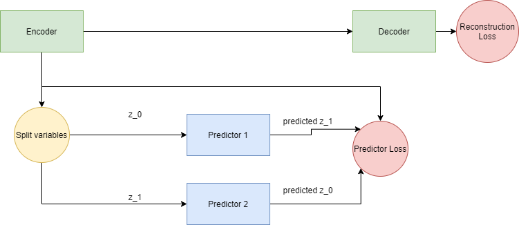
Figure 1: The basic setup of predictability minimization for independent component analysis.
There is an encoder-decoder, which wants to encode the data and reconstruct it as best as possible. There is also a collection of predictors, that get the latent code of the encoder as their input, except for one code value, and these predictors have to predict the value of this missing unit.
The encoder is driven to put as much useful information in the code representation as possible (so that the decoder may use it to reconstruct the input). While doing this, the encoder also tries to maximize the loss of the collection of predictors: it encodes the information such that knowing the value of 1 code unit is of no use for predicting another. At the end of the process, what we are left with is an encoder that will perform independent component analysis on (data similar to) the training data.
Let us get to the code. First we define a Dataset that will give use the 4 sequences that we want to perform independent component analysis on.
class UniformDataset(Dataset):
    """Uniform dataset."""

    def __init__(self):
        self.uniform_data = np.random.uniform(size=(4, 4))

    def __len__(self):
        return len(self.uniform_data)

    def __getitem__(self, idx):
        return self.uniform_data[idx]
A typical set of 4 data points looks like this:
>> [[0.08641456 0.19421044 0.88229338 0.0361495 ]
>>  [0.01163331 0.33199609 0.38802061 0.66070623]
>>  [0.5881097  0.97043498 0.98881562 0.11357908]
>>  [0.94657677 0.69272661 0.26470928 0.88500763]]
The original paper claimed that given two code units, with the specific setup of losses that we will clarify, the encoder will learn to encode these 4 sequences in binary notation. This means that there will be 4 different values for the length-2 latent code: 00, 01, 10 and 11.
Now we define the Predictability Minimization class, which will host the neural networks that will be adversarially optimizing their losses. The point of this code is to be clear, but it can definitely be expanded to a case with a larger code and more predictor units.
class PM(nn.Module):

    def __init__(self):
        super(PM, self).__init__()

        # encoder
        self.encoder = nn.Sequential(
            nn.Linear(4, 40),
            nn.ReLU(),
            nn.Linear(40, 2),
            nn.Sigmoid()
        )

        # decoder

        self.decoder = nn.Sequential(
            nn.Linear(2, 40),
            nn.ReLU(),
            nn.Linear(40, 4)
        )

        # predictor 1

        self.predictor_1 = nn.Sequential(
            nn.Linear(1, 40),
            nn.ReLU(),
            nn.Linear(40, 1),
            nn.Sigmoid()
        )

        # predictor 2

        self.predictor_2 = nn.Sequential(
            nn.Linear(1, 40),
            nn.ReLU(),
            nn.Linear(40, 1),
            nn.Sigmoid()
        )

    def forward(self, x):
        code = self.encoder(x)

        reconstruction = self.decoder(code)

        code1 = torch.tensor(code)[:, 1].reshape(4, 1)
        code0 = torch.tensor(code)[:, 0].reshape(4, 1)

        pred1 = self.predictor_1(code1).to(device)
        pred2 = self.predictor_2(code0).to(device)

        return code, pred1, pred2, reconstruction
On to the loss terms: we have a standard mean square error loss for the autoencoder part:
\[I = \frac{1}{n} \sum_{n=1}^N (Y_{true} - Y_{pred})^2\]In addition to this, we compute the mean square error between the value of the code units and the predictor unit’s estimates of what they are. This is called \(V_c\) in the original paper.
\[V_c = \frac{1}{n} \sum_{n=1}^N (Y_{code} - Y_{predicted})^2\]The code units try to maximize this loss (as they supply the first term) while the predictor units try to minimize this loss (they supply the second term).
The following piece of code defines the losses and optimizers:
train_dataset = UniformDataset()

# device = torch.device('cuda')
device = 'cpu'
num_epochs = 10000
batch_size = 4
learning_rate = 0.01

# Data loader
train_loader = torch.utils.data.DataLoader(dataset=train_dataset,
                                           batch_size=batch_size,
                                           shuffle=True)

model = PM().to(device)

# Loss that measures how close the predictions of the
# predictor units are to the actual code units
criterion = nn.MSELoss()

# Loss for the auto encode structure
reconstruction_criterion = nn.MSELoss()

# This optimizer governs the code units
code_optimizer = torch.optim.Adam(list(model.encoder.parameters()), lr=learning_rate)

# This optimizer governs the decoder
reconstruction_optimizer = torch.optim.Adam(list(model.decoder.parameters()) +
                                           list(model.encoder.parameters()),
                                           lr=learning_rate)

# This optimizer governs the predictors, that enforce the independence of the code units
prediction_optimizer = torch.optim.Adam(list(model.predictor_1.parameters()) +
                                       list(model.predictor_2.parameters()),
                                       lr=2 * learning_rate)
Note especially that we are using three different optimizers: this is not optimal for stability and we will be following up on this in a future post.
The code that actually trains the model is the following:
# Train the model
total_step = len(train_loader)
for epoch in range(num_epochs):
    for i, samples in enumerate(train_loader):
        # Move tensors to the configured device
        seqs = samples.float().to(device)
        # print(seqs.shape)
        # Forward pass
        code, pred_1, pred_2, reconstruction = model.forward(seqs)
        # print(code.shape)
        preds = torch.cat([pred_1, pred_2], dim=1).to(device)
        # print(preds.shape)

        # The reconstruction loss
        recon_loss = 1 * reconstruction_criterion(seqs, reconstruction)

        # The predictive layers want to minimize the
        # predictor loss (predict the code units from each other) while
        # The code units want to maximize that the predictor loss

        predictor_loss = criterion(code, preds)
        code_loss = -1 * predictor_loss

        prediction_optimizer.zero_grad()
        predictor_loss.backward(retain_graph=True)
        prediction_optimizer.step()

        reconstruction_optimizer.zero_grad()
        recon_loss.backward(retain_graph=True)
        reconstruction_optimizer.step()

        code_optimizer.zero_grad()
        code_loss.backward(retain_graph=True)
        code_optimizer.step()
After training the network, the code units give the following values for the 4 sequences:
tensor([[9.9999e-01, 2.1293e-11],
        [1.9540e-08, 9.9998e-01],
        [8.5616e-06, 2.4651e-05],
        [1.0000e+00, 1.0000e+00]])
When rounded, this gives the following values:
tensor([[1, 0],
        [0, 1],
        [0, 0],
        [1, 1]])
That does look like a binary code!